`stat_movingaverages` is a `ggplot2` layer that allows you to plot moving averages on a `ggplot2` plot either by providing the column names `ggplot2::aes` of the previously calculated metrics.
You are free to use whatever algorithm you desire; the result will be two line plots one for a short moving average and one for a long moving average.
To use this layer provide `ggplot2::aes` values for `x` (datetime x-axis) and `short` and `long` (y-axis).
See examples for more details.
Usage
stat_movingaverages(
  mapping = NULL,
  data = NULL,
  geom = "line",
  position = "identity",
  na.rm = TRUE,
  show.legend = NA,
  inherit.aes = TRUE,
  linewidth = 1.75,
  alpha = 0.75,
  colour = list(short = "yellow", long = "purple"),
  ...
)
Arguments
- mapping
A `ggplot2::aes` object (required - default `NULL`).
- data
A `data.table` object (required - default `NULL`).
- linewidth
A `numeric` vector of length one; the width of the line (optional - default `1.75`).
- alpha
A `numeric` vector of length one; the alpha of the line (optional - default `0.75`).
- colour
A named or unnamed `list` with three elements "short" and "long". These are the colours for the short and long moving averages (optional - default `list(short = "red", long = "blue")`).
Details
This is a `ggplot2` extension; it is used with the `+` operator for adding a layer to a `ggplot2` object.
Aesthetics
stat_movingaverages understands the following aesthetics (required aesthetics are in bold):
x -- datetime (x-axis)
short -- the values for the short moving average (y-axis).
long -- the values for the long moving average (y-axis)
Examples
# get some financial data
# kucoin is private package - you can use any data source
ticker <- "BTC/USDT"
dt <- kucoin::get_market_data(
symbols = ticker,
from = "2022-11-28 15:29:43 EST", # lubridate::now() - lubridate::days(7),
to = "2022-12-05 15:29:31 EST", # lubridate::now(),
frequency = "1 hour"
)
dt
#> symbol datetime open high low close volume
#> <char> <POSc> <num> <num> <num> <num> <num>
#> 1: BTC/USDT 2022-11-28 15:00:00 16215.3 16233.6 16126.0 16144.1 327.8979
#> 2: BTC/USDT 2022-11-28 16:00:00 16144.1 16382.6 16000.0 16305.9 837.5801
#> 3: BTC/USDT 2022-11-28 17:00:00 16305.9 16382.0 16195.4 16205.4 507.8351
#> 4: BTC/USDT 2022-11-28 18:00:00 16206.1 16230.7 16146.5 16162.6 252.3387
#> 5: BTC/USDT 2022-11-28 19:00:00 16161.7 16253.3 16150.1 16220.9 225.4121
#> ---
#> 165: BTC/USDT 2022-12-05 11:00:00 17295.2 17314.3 17283.8 17312.0 176.8633
#> 166: BTC/USDT 2022-12-05 12:00:00 17312.0 17318.6 17230.5 17254.5 199.6922
#> 167: BTC/USDT 2022-12-05 13:00:00 17254.5 17282.5 17208.1 17229.7 105.2655
#> 168: BTC/USDT 2022-12-05 14:00:00 17229.8 17241.4 17175.1 17205.2 140.4375
#> 169: BTC/USDT 2022-12-05 15:00:00 17205.1 17205.1 17021.6 17083.0 504.9158
#> turnover
#> <num>
#> 1: 5301836
#> 2: 13557348
#> 3: 8270203
#> 4: 4082464
#> 5: 3653147
#> ---
#> 165: 3058929
#> 166: 3447960
#> 167: 1815447
#> 168: 2416907
#> 169: 8630174
# we need a function that calculates the indicator for us
# typically I like to write my own functions in C++; in this case we will use TTR's
# the stat expects a named list to be returned - we redefine ttr
ema <- function(close, n = 2, wilder = TRUE) {
return(as.list(as.data.frame(TTR::EMA(close, n = n, wilder = wilder))))
}
# calculate the short and long moving averages
dt[, ema_short := ema(close, n = 10, wilder = TRUE)]
#> symbol datetime open high low close volume
#> <char> <POSc> <num> <num> <num> <num> <num>
#> 1: BTC/USDT 2022-11-28 15:00:00 16215.3 16233.6 16126.0 16144.1 327.8979
#> 2: BTC/USDT 2022-11-28 16:00:00 16144.1 16382.6 16000.0 16305.9 837.5801
#> 3: BTC/USDT 2022-11-28 17:00:00 16305.9 16382.0 16195.4 16205.4 507.8351
#> 4: BTC/USDT 2022-11-28 18:00:00 16206.1 16230.7 16146.5 16162.6 252.3387
#> 5: BTC/USDT 2022-11-28 19:00:00 16161.7 16253.3 16150.1 16220.9 225.4121
#> ---
#> 165: BTC/USDT 2022-12-05 11:00:00 17295.2 17314.3 17283.8 17312.0 176.8633
#> 166: BTC/USDT 2022-12-05 12:00:00 17312.0 17318.6 17230.5 17254.5 199.6922
#> 167: BTC/USDT 2022-12-05 13:00:00 17254.5 17282.5 17208.1 17229.7 105.2655
#> 168: BTC/USDT 2022-12-05 14:00:00 17229.8 17241.4 17175.1 17205.2 140.4375
#> 169: BTC/USDT 2022-12-05 15:00:00 17205.1 17205.1 17021.6 17083.0 504.9158
#> turnover ema_short
#> <num> <num>
#> 1: 5301836 NA
#> 2: 13557348 NA
#> 3: 8270203 NA
#> 4: 4082464 NA
#> 5: 3653147 NA
#> ---
#> 165: 3058929 17226.35
#> 166: 3447960 17229.17
#> 167: 1815447 17229.22
#> 168: 2416907 17226.82
#> 169: 8630174 17212.44
dt[, ema_long := ema(close, n = 50, wilder = TRUE)]
#> symbol datetime open high low close volume
#> <char> <POSc> <num> <num> <num> <num> <num>
#> 1: BTC/USDT 2022-11-28 15:00:00 16215.3 16233.6 16126.0 16144.1 327.8979
#> 2: BTC/USDT 2022-11-28 16:00:00 16144.1 16382.6 16000.0 16305.9 837.5801
#> 3: BTC/USDT 2022-11-28 17:00:00 16305.9 16382.0 16195.4 16205.4 507.8351
#> 4: BTC/USDT 2022-11-28 18:00:00 16206.1 16230.7 16146.5 16162.6 252.3387
#> 5: BTC/USDT 2022-11-28 19:00:00 16161.7 16253.3 16150.1 16220.9 225.4121
#> ---
#> 165: BTC/USDT 2022-12-05 11:00:00 17295.2 17314.3 17283.8 17312.0 176.8633
#> 166: BTC/USDT 2022-12-05 12:00:00 17312.0 17318.6 17230.5 17254.5 199.6922
#> 167: BTC/USDT 2022-12-05 13:00:00 17254.5 17282.5 17208.1 17229.7 105.2655
#> 168: BTC/USDT 2022-12-05 14:00:00 17229.8 17241.4 17175.1 17205.2 140.4375
#> 169: BTC/USDT 2022-12-05 15:00:00 17205.1 17205.1 17021.6 17083.0 504.9158
#> turnover ema_short ema_long
#> <num> <num> <num>
#> 1: 5301836 NA NA
#> 2: 13557348 NA NA
#> 3: 8270203 NA NA
#> 4: 4082464 NA NA
#> 5: 3653147 NA NA
#> ---
#> 165: 3058929 17226.35 17017.34
#> 166: 3447960 17229.17 17022.08
#> 167: 1815447 17229.22 17026.23
#> 168: 2416907 17226.82 17029.81
#> 169: 8630174 17212.44 17030.88
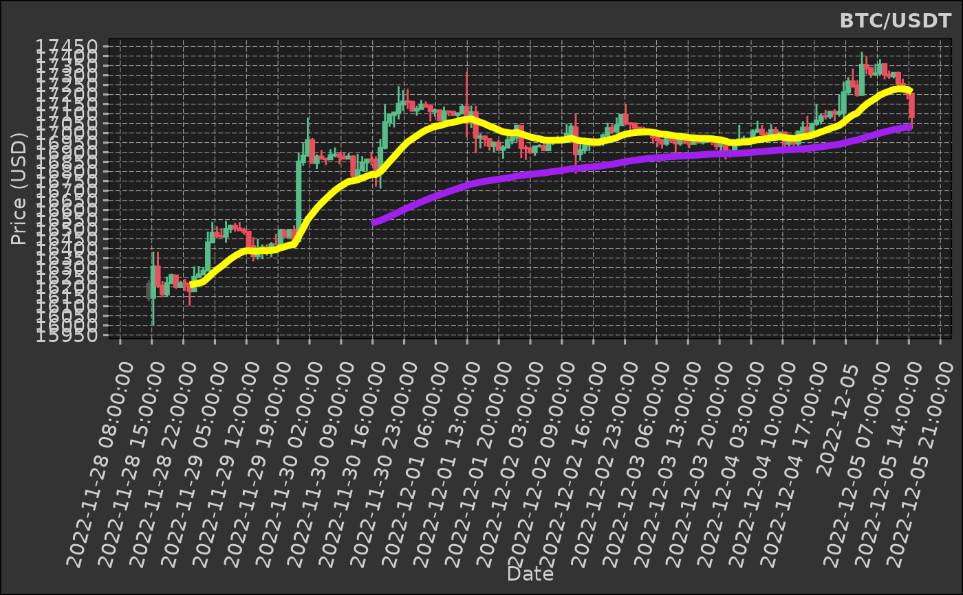
dt |>
ggplot2::ggplot(ggplot2::aes(
x = datetime,
open = open,
close = close,
high = high,
low = low,
group = symbol
)) +
## ------------------------------------
dmplot::stat_candlestick() +
## ------------------------------------
# provide the colnames to the calculated indicators as aes values
dmplot::stat_movingaverages(ggplot2::aes(short = ema_short, long = ema_long), alpha = list(mavg = 0.5)) +
## ------------------------------------
ggplot2::scale_x_continuous(n.breaks = 25, labels = \(x) {
lubridate::floor_date(lubridate::as_datetime(x), "hours")
}) +
ggplot2::scale_y_continuous(n.breaks = 25) +
ggplot2::labs(
title = ticker,
x = "Date",
y = "Price (USD)"
) +
dmplot::theme_dereck_dark() +
ggplot2::theme(
axis.text.x = ggplot2::element_text(angle = 75, vjust = 0.925, hjust = 0.975),
panel.grid.minor = ggplot2::element_blank()
)